Diffusion Models (DDPM)

In this first post of my blog, I’m going to try to share everything I’ve learned about diffusion models. Specifically, we’ll focus on the original paper that introduced Denoising Diffusion Probabilistic Models (DDPM) - you can find the reference at the end of this post. Besides reading this entry, I encourage you to read the original paper as well; it’s fascinating and can help you better understand the model, especially if you use this blog and other resources I mention below, which can be even more useful!

If you’re only looking for a basic introduction or a quick overview of diffusion models, this post might be too detailed to start with. Here I talk about what I would have liked to know when I already had an idea of how these models worked, but wanted to understand in depth their operation and underlying mathematics. If that’s your case, definitely check out the additional resources I share at the end.

Initial Summary

Diffusion models are a type of generative model. This means that a neural network is trained to learn the distribution of some data, so that it can create new instances that fit within that distribution. The key to these models lies in a change in their training and generation process, rather than in the model structure itself. So, basically, DDPMs are a different way of training and generating data, but they don’t involve a new network architecture.

What a diffusion model is NOT

However, rather than explaining what a diffusion model is, I find it interesting to start by defining what it is NOT.

DDPMs are not:

• A new model architecture.
• A new type of neural layer.

This is also similar in the case of GANs (Generative Adversarial Networks), since the heart of their change lies in the training algorithm and translates into the use of an adversarial loss function to adjust their parameters.

Advantages and disadvantages

The 3 pillars of generative models and their respective strengths

Basically, a diffusion model is one of the three pillars of generation techniques that exist today. And it’s often said that each pillar is good at 2 points, but very bad at the other.

Specifically, diffusion models have the following advantages:

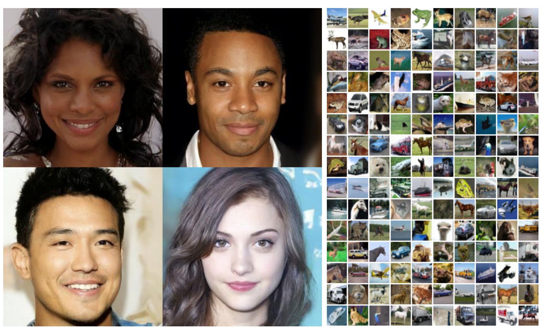
• Generate new samples of very high quality.
• Can learn multiple distributions at once.

But in addition, over GANs, they have the advantage of:

• Much more stable convergence by not having two models interacting with each other.
• They don’t suffer from the famous model collapse problem.

However, their main disadvantage is the slowness of generation.

In the original paper on Denoising Diffusion Imputation Models (DDIM), it’s mentioned that creating 50,000 32x32 pixel images using GANs on an Nvidia 2080 Ti card takes less than a minute. However, with diffusion models, we’re talking about about 1000 hours for the same task.

Although for a long time diffusion models have been considered one of the essential pillars of generative models, lately this rule of the 3 pillars is becoming less clear. Thanks to improvements like those introduced by DDIMs, progress is being made towards overcoming speed barriers and opening new paths for their practical use, breaking the disadvantage in the generation speed of diffusion models.

General Operation

A diffusion model basically takes original data and gradually decomposes it, corrupting it with noise until all that remains is a cloud of pure noise, that is, data that follows a standard normal distribution, which mathematically speaking is represented as: $\mathcal{N}(0, 1)$.

This process of adding noise is performed gradually, following a series of predefined steps. This can be described using what we call a Markov chain of $T$ steps. At the beginning, you have an initial sample, which we call $x_0$, and at the end of the process, you reach $x_t$, the point where the data has already been completely transformed into noise, satisfying that $x_t \sim \mathcal{N}(0, 1)$.

Markov chain. Moving forward through it destroys the sample, but if we go backwards it returns to its original state

To ensure that our data transforms correctly into pure noise of the form $\mathcal{N}(0, 1)$ throughout the Markov chain, we carefully adjust how much noise we add at each step. This is done through a parameter called $\beta$. This parameter is not fixed; it changes progressively until we achieve that our data becomes completely noise, reaching the state $x_t \sim \mathcal{N}(0, 1)$. Therefore, at each step of our chain we have a specific $\beta_t$.

We can think of $\beta_t$ as being under the control of something we call the Scheduler, which would be like a Python object in charge of managing how $\beta$ evolves over time. Think of it as a list that keeps track of how the values of $\beta_t$ change for each instant $t$. And when we need to know the value of $\beta$ at a specific moment, we simply ask the Scheduler with something like scheduler.get_beta(t). Although there are several strategies that the Scheduler can use to define these values, the original approach proposed in the paper is to use a linear Scheduler.

We go from the initial distribution to a noise mask

The scheduler modifying the mean of the distribution along the chain. In the first case the linear one was presented, the cosine one was presented later

So, what we seek to do is train a model that is capable of guessing how much noise we have added at the current moment. If we manage to correctly predict this noise and remove it, we should be able to return to the previous state of our data. This process, done step by step iteratively, would allow us, in theory, to use our model to predict the noise masks at each stage and, thus, completely reverse the process, going from $x_t$ to $x_0$.

Loop to traverse the Markov chain backwards and generate a new sample. It will be explained in more detail later

Main Components of Diffusion Models

Having said this, to properly understand diffusion models there are 5 key elements that we need to understand:

1. The Scheduler

2. The forward process $q(x_t

   x_{t-1})$

3. The posterior of the forward process $q(x_{t-1}

   x_t, x_0)$

4. The backward/reverse process $p_{\theta}(x_{t-1}

   x_t)$

5. The loss function

Scheduler

As we have seen previously, the amount of noise we add at each stage of our Markov chain varies; it’s not a fixed value. This is carefully designed to ensure that, at the end of the process, we end up with something that resembles $x_t \sim \mathcal{N}(0, 1)$. If we chose to add a constant amount of noise at each step, the variability of our distribution would skyrocket due to the accumulation of this noise, so it’s crucial to adjust the intensity of the noise we add gradually. This is where the Scheduler and the famous $\beta_t$ come into play, which determines how much noise to add at each step.

In essence, at the beginning of each step we generate a new set of noise according to $\epsilon \sim \mathcal{N}(0, 1)$, and we adjust its intensity using $\beta_t$. We’ll delve deeper into this process later, but for now, it’s vital to understand the role of the Scheduler, the function of $\beta_t$, and the fact that the amount of noise we introduce varies at each step.

Forward/Diffusion process $q(x_t|x_{t-1})$

Okay, we’ve established that we’re going to corrupt the initial samples along a Markov chain in which we’re going to progressively add noise, but how is this done?

The paper offers us a specific formula, Formula \ref{eq:foward}, that guides us on how to advance from a state $t-1$ to the next $t$. This formula is our roadmap to be able to advance through the chain.

\[\begin{equation} q(x_t|x_{t-1}) = \mathcal{N}(x_t; \underbrace{\sqrt{1-\beta_t}x_{t-1}}_{\mu}, \underbrace{\beta_t I}_{\sigma^2}) \label{eq:foward} \end{equation}\]

Don’t worry if Formula \ref{eq:foward} seems a bit convoluted to you. Basically, what it does is apply a normal distribution with a mean $\mu = \sqrt{1-\beta_t}x_{t-1}$ and a variance $\sigma^2=\beta_t I$. In fact, I prefer a more explicit version of this formula, which the original paper also presents. Let’s define it starting from the base, with the normal distribution formula:

\[\begin{equation} \mathcal{N}(\mu, \sigma^2) = \mu + \sigma ·\epsilon \label{eq:normal} \end{equation}\] \[\epsilon \sim \mathcal{N}(0,1)\]

With the normal distribution definition established in Formula \ref{eq:normal}, we can reformulate Formula \ref{eq:foward}. This new version of the formula takes into account the specific parameters of the normal distribution to apply noise to our samples along the Markov chain.

\[\begin{equation} q(x_t|x_{t-1}) = \sqrt{1-\beta_t}x_{t-1} + \sqrt{\beta_t}\epsilon \label{eq:foward_explicit} \end{equation}\]

With Formula \ref{eq:foward_explicit}, to reach any point $t$, we only need to apply it iteratively from $t=0$, as shown below:

\[\begin{equation} q(x_{1:T}|x_0):=\prod^T_{t=1}{q(x_t|x_{t-1})} \end{equation}\]

Indeed, following this step-by-step method is not practical at all, especially considering that during training we need to evaluate our network with different values of $t$. Having to traverse the entire chain to reach each specific step represents an enormous computational cost. For this reason, it’s necessary to modify the formula to obtain a new one that allows us to jump directly from $x_0$ to $x_t$, without having to go through each intermediate step. Let’s start by defining the following new variables to simplify this process:

\[\begin{equation} \alpha_t = 1 - \beta_t \end{equation}\] \[\overline{\alpha_t} = \prod^t_{s=1}\alpha_t\]

Thus, $\overline{\alpha_t}$ somehow encapsulates the accumulation of all previous $\beta$s in the chain. This allows us to reformulate Formula \ref{eq:foward_explicit} in a more efficient and direct way, facilitating the jump from $x_0$ to $x_t$:

\[\begin{equation} q(x_t|x_0) = \sqrt{\overline{\alpha_t}}x_0 + \sqrt{1-\overline{\alpha_t}}\epsilon \label{eq:foward_xoxt} \end{equation}\]

With Formula \ref{eq:foward_xoxt} at our disposal, we now have an efficient mechanism to transform any original sample $x_0$ into its corrupted version $x_t$, corresponding to step $t$ of the Markov chain, using a single jump. This greatly simplifies the process and makes the concept of “Forward process” more accessible. So, from now on, when we talk about the forward process, we will be referring specifically to $q(x_t

x_0)$ as defined by Formula \ref{eq:foward_xoxt}.

Posterior of forward process $q(x_{t-1}|x_t, x_0)$

Okay, now let’s focus on what’s truly crucial: the reverse process. We need to discover how we can reverse the process, that is, how to go backwards through the Markov chain to recover the original sample starting from its corrupted state.

\[\begin{equation} q(x_t|x_{t-1}, x_0) = \frac{\overbrace{q(x_{t-1}|x_{t}, x_0)}^{\text{posterior}}q(x_{t}|x_0)}{q(x_{t-1}| x_0)} \label{eq:posterior_bayes} \end{equation}\]

To achieve this backtracking in the Markov chain, applying Bayes’ theorem (detail you can find expanded in Formula \ref{eq:posterior_bayes}), we manage to derive this “posterior”. This defines how to obtain the previous step in the chain, conditioned by the current step and by the original sample. The definition of this posterior is as follows:

\[\begin{equation} q(x_{t-1}|x_t, x_0) = \mathcal{N}(x_{t-1};\tilde{\mu}_t(x_t,x_0),\tilde{\beta}_tI) \label{eq:posterior} \end{equation}\] \[\begin{equation} \tilde{\mu}_t(x_t,x_0) := \frac{\sqrt{\overline{\alpha}_{t-1}}\beta_t}{1-\overline{\alpha}_t}x_0 + \frac{\sqrt{\alpha_{t}}(1-\overline{\alpha}_{t-1})}{1-\overline{\alpha}_t}x_t \label{eq:mu_tilde} \end{equation}\] \[\begin{equation} \tilde{\beta}_t:= \frac{1-\overline{\alpha}_{t-1}}{1-\overline{\alpha_t}}\beta_t \label{eq:beta_tilde} \end{equation}\]

It’s true that depending on $x_0$ in the formulas, especially Formulas \ref{eq:posterior} and \ref{eq:mu_tilde}, can be somewhat uncomfortable. This dependency becomes even more problematic later during the generation of new samples, since at that time we don’t have $x_0$ available. However, there’s a trick we can use to get around this inconvenience. If we consider that $q(x_t

x_0) = x_t$, we can solve Formula \ref{eq:foward_xoxt} to eliminate $x_0$. Doing this, we derive the following new formula:

\[\begin{equation} x_0 = \frac{1}{\sqrt{\overline{\alpha}_t}}(x_t - \frac{1-\alpha}{\sqrt{1-\overline{\alpha}_t}}\epsilon) \label{eq:x_0_despejado} \end{equation}\]

And if we apply Formula \ref{eq:x_0_despejado} to Formula \ref{eq:mu_tilde} we get the following:

\[\begin{equation} \tilde{\mu}(x_t,x_0) = \frac{1}{\sqrt{\alpha}}(x_t-\frac{\beta_t}{\sqrt{1-\overline{\alpha}}_t}\epsilon) \label{eq:mu_tilde_despejada} \end{equation}\]

With this we already have almost everything done, we have to perform a final cleanup in Formula \ref{eq:posterior}, for this we’re going to do the following:

To give the final touches to Formula \ref{eq:posterior} and leave it ready for use, we’re going to refine it a bit more with three key steps:

1. Apply Formula \ref{eq:normal} that defines the normal
2. Apply the definition of $\tilde{\mu}(x_t,x_0)$ that we obtained in Formula \ref{eq:mu_tilde_despejada}

3. Perform a small substitution to simplify a bit more, since we know that $x_t = q(x_{t-1}

   x_t, x_0)$

With these adjustments, we manage to refine our formula, making it more accessible:

\[\begin{equation} x_{t-1} = \frac{1}{\sqrt{\alpha}}(x_t-\frac{\beta_t}{\sqrt{1-\overline{\alpha}}}\epsilon_t) + \sqrt{\beta_t}\epsilon \label{eq:posterior_clean} \end{equation}\]

With Formula \ref{eq:posterior_clean} in hand, we’re prepared to go backwards through the Markov chain. But, there’s an important small detail to point out: the distinction between two types of $\epsilon$, which I’ve differentiated as $\epsilon_t$ and simply $\epsilon$, to avoid confusion. Understanding the role of each one is crucial:

1. $\epsilon$ represents the noise that is introduced when applying the normal. This is the specific noise that is added in a given step to adjust to the definition of the normal distribution that we apply when going backwards.

2. $\epsilon_t$ is the critical element in this context. It represents the total sum of noise applied to $x_0$ to transform it into $x_t$. This concept is fundamental because it encapsulates the entire diffusion process, reflecting the accumulation of noise along the steps until reaching the current state.

Backwards process $p_{\theta}(x_{t-1}|x_t)$

Now that we understand how to navigate the Markov chain, both forward and backward, the main objective focuses on enabling our model to perform this reverse process efficiently. What we seek is that $p_{\theta}(x_{t-1}

x_t)$ learns to imitate the process of $q(x_{t-1}

x_t, x_0)$.

Initially, the definition of the reverse process is established as follows:

\[\begin{equation} p(x_{t-1}|x_t) = \mathcal{N}(x_{t-1}; \mu_\theta(x_t, t),\Sigma_\theta(x_t, t)) \label{eq:backward_full} \end{equation}\]

Indeed, analogously to Formula \ref{eq:posterior}, our objective is to be able to predict the distribution of the sample in the previous step. This implies that, ideally, we should have a model (or even two different ones) that can predict both the mean $\mu_\theta(x_t, t)$ and the variance $\Sigma_\theta(x_t, t)$ of the normal distribution in question. However, the authors of the original paper discovered that omitting the prediction of $\Sigma_\theta(x_t, t)$ led to more efficient results. Since the variance is already determined by the Scheduler, we can dispense with predicting it, which simplifies the process (although subsequent research has found advantages in predicting $\Sigma_\theta(x_t, t)$). With this adjustment, the formulation of the reverse process is considerably simplified:

\[\begin{equation} p(x_{t-1}|x_t) = \mathcal{N}(x_{t-1}; \mu_\theta(x_t, t), \beta_t I) \label{eq:backward_mu} \end{equation}\]

So, at this point the mean we have to predict is the following:

\[\begin{equation} \mu_\theta(x_t, t) = \frac{1}{\sqrt{\alpha_t}}(x_t - \frac{\beta_t}{\sqrt{1 - \overline{\alpha_t}}}\epsilon_\theta(x_t, t)) \label{eq:mu_prediction} \end{equation}\]

That’s right, at the core, the crucial parameter to predict becomes $\epsilon_\theta(x_t, t)$, which effectively represents the noise that has been accumulating throughout the entire chain up to point $t$. This tells us how the original sample has been modified to reach this specific state of this step in the chain. By correctly predicting this noise, we can adjust it for the current step with the factor $\frac{\beta_t}{\sqrt{1 - \overline{\alpha_t}}}$, allowing us to eliminate it gradually and, therefore, advance in reverse through the chain.

Integrating what we’ve seen, if we reconstruct Formula \ref{eq:backward_mu} with the information from Formula \ref{eq:mu_prediction} and the normal distribution definition from Formula \ref{eq:normal}, and we consider that $x_{t-1} = p(x_{t-1}

x_t)$, we arrive at the definitive equation that allows us to go backwards step by step along the Markov chain. This process shows us how, through precise prediction of noise at each stage, we can go backwards along the diffusion path to recover the original sample from its corrupted state.

\[\begin{equation} x_{t-1} = \frac{1}{\sqrt{\alpha_t}}(x_t - \frac{\beta_t}{\sqrt{1 - \overline{\alpha_t}}}\epsilon_\theta(x_t, t)) + \sqrt{\beta_t}\epsilon \label{eq:backwards_final} \end{equation}\]

Once again, two different $\epsilon$s appear, let’s define them again:

1. $\epsilon$ is the noise that is applied to fulfill the definition of the normal.
2. $\epsilon_\theta(x_t, t)$ is the noise value predicted by the model to calculate the mean. This value represents the accumulated noise that has been applied up to point $t$ in the chain. Predicting this noise accurately is essential to be able to reverse the diffusion process, eliminating the added noise and recovering the original sample as we go backwards through the chain.

Alternative definition with $q(x_{t-1}|x_t, \hat{x}_0)$

Although Formula \ref{eq:backwards_final} is the one commonly used and most discussed when we talk about diffusion models, it’s possible that on some occasions you’ll encounter that $ q(x_{t-1}

x_t, \hat{x}_0) $ is applied to go backwards along the chain.

Actually, $$ q(x_{t-1}

x_t, \hat{x}0) \(and\) p(x{t-1}

x_t) $$ work in a very similar way, with the main difference being that the first one doesn’t explicitly eliminate $x_0$ from the equation, as is done in the process we’ve already seen that goes from Formula \ref{eq:posterior} to Formula \ref{eq:posterior_clean}.

If you encounter this formula, there’s no reason to worry too much. The only thing that’s done is to generate $\hat{x}_0$, which basically involves estimating the original sample $x_0$ based on the current state $x_t$ and the noise accumulated up to that point:

\[\begin{equation} \hat{x}_0 = \frac{1}{\sqrt{\overline{\alpha_t}}}(x_t - \sqrt{1-\overline{\alpha_t}}\epsilon_\theta(x_t, t)) \label{eq:x_pred} \end{equation}\]

You can apply this or simply understand that they are really the same formulas and continue using Formula \ref{eq:backwards_final} with confidence, the final result will be the same.

Important Considerations

The importance of t

The need to include time $t$ as a parameter in the models is crucial, as we have observed throughout this post about diffusion models. The reason behind this is that the noise added at each step of the Markov chain is not uniform, which means the model needs to know at which specific point it is located to adequately estimate the corresponding noise.

Difficulty in maintaining $x_0 \in [-1, 1]$

One of the challenges with diffusion models is the difficulty of maintaining sample values within the range of [-1, 1] as noise is removed to go backwards through the chain. There are several strategies to address this, although not all are equally effective. A common tactic is to limit the maximum values that samples can reach, but this may be insufficient. Another option is to normalize the samples again, which can be a more effective solution for this problem.

In the last step we don’t add noise

It’s important to note, as indicated in Formula \ref{eq:backwards_final}, that although we generally add noise to comply with the definitions of normal distributions when going backwards through the chain, we don’t add noise in the last step, that is, when going from $x_1$ to $x_0$. This is logical, since the final objective is to recover the original sample as it was, without introducing any additional alteration at this critical point of the process.

Loss Function

The key to teaching our model to navigate efficiently through the Markov chain and go backwards accurately lies in the loss function we use during training. Ideally, we would want this function to be the log-likelihood of $p_\theta(x_0)$, which would imply traversing the entire chain for each training batch, an extremely expensive and practically unfeasible process, as the paper rightly points out by defining it as an intractable process.

To circumvent this obstacle, we rely on the concept of the Variational Lower Bound, which is always at least less than the log-likelihood. By optimizing this function, we are indirectly improving the log-likelihood, since the Variational Lower Bound always sits below the latter.

This relationship is clearly illustrated in the following image, which shows that by optimizing this function, we actually improve the log-likelihood. This approach allows us to train our model efficiently, focusing on improving this lower bound with the confidence that, by doing so, we are also improving the log-likelihood of our model.

Example of log-likelihood and Variational Lower Bound. The latter will always be below log-likelihood, and therefore, improving it, ends up improving the log-likelihood.

Basically, this is defined with the following formula:

\[\begin{equation} \mathbb{E}[\underbrace{-\log{p_\theta(x_0)}}_{NLL}]\le\mathbb{E}_q[-\underbrace{\log p_\theta(x_0|x_1)}_{L_0} + \sum_{t>1}\underbrace{D_{KL}(q(x_{t-1}|x_t,x_0) || p_\theta(x_{t-1}|x_t))}_{L_{t-1}} +\underbrace{D_{KL}(q(x_T|x_0) || p(x_T))}_{L_T}] \label{eq:elbo} \end{equation}\]

The equation we have before us may seem like a challenge at first glance, but let’s break it down step by step to make it more understandable:

• $NLL$: It’s the negative log-likelihood, it’s established that it will always be equal to or less than what’s found to the right of the inequality.

From here, the approach focuses on comparing how similar the real distributions $q$ are to what our model $p_\theta$ manages to learn. This comparison is made through KL divergence. So:

• $L_0$: represents how the negative log-likelihood is measured in the first step of the chain.
• $L_{t-1}$: refers to the likelihood of the intermediate steps of the chain.
• $L_{T}$: is about the last step of the chain. Here, basically, we have two noise distributions $\sim\mathcal{N}(0,1)$, dictated by the Scheduler, which allows us to simplify and exclude this part from our equation.

Despite everything, you don’t have to be afraid of this piece of formula. In the end, what really matters to ensure a good approximation in the reconstruction process is an accurate estimation of $\epsilon_\theta(x_t, t)$. With this idea in mind and doing a “cleanup” of Formula \ref{eq:elbo}, we obtain the following simplification:

\[\begin{equation} \mathcal{L} = \mathbb{E}_{t, x_o, \epsilon} [||\epsilon - \epsilon_\theta(x_t, t)||^2] \label{eq:loss} \end{equation}\]

In the end, what we’re left with as a loss function is the MSE between the real error and the predicted one, something undoubtedly much more manageable.

Algorithms

Now that we’ve internalized the mathematical foundations behind diffusion models, it’s time to take a look at the algorithms that make them work. Unlike GANs, here we’ll find a more marked distinction between the algorithm used for training and the one used for generation.

Training

Training algorithm

The operation is as follows:

1. We select a training batch
2. We randomly generate a different value of $t$ for each sample
3. We generate the $x_t$ according to the $t$ that each one got and save the noise matrix of each one.
4. We use our model to predict the noise matrix based on $x_t$ and $t$
5. We calculate the MSE between the real noise and the predicted one and backpropagate the error.

Generation

Sample generation algorithm

It’s a bit different from the previous one, but basically what we have to do is the following:

1. Generate a batch with as many random noise matrices as samples we want to generate. These will be our $x_t$
2. Perform the prediction of the noise they have by using our model using $x_t$ and $t$.
3. Reconstruct $x_{t-1}$ with the predicted noise.
4. Repeat until we’ve traversed the entire chain.

In this way, starting from random noise, our model ends up generating completely new samples.

UNET: The First Architecture Used

Unet representation

The first architecture used with diffusion models was the Unet, since it’s a very famous architecture in the field of computer vision. After all, since this first paper generated images, using this model meant having a very good starting point.

But when we introduce the Unet into the universe of diffusion models, there’s an interesting twist. It’s not simply copy and paste; the implementation has a special touch so that everything fits with the diffusion process, as can be seen in the following image that would represent a top view of the model architecture:

Unet representation from above

The value of $t$, or the step in the Markov chain, is not introduced into the network directly. Instead, a technique inspired by transformers called positional encoding is used, where $t$ is encoded through multiple sinusoidal signals. This method, better known for its use in transformer architecture to maintain the notion of position in text sequences, is here adapted to inject the temporal dimension about the step we’re at in the chain within the network.

This encoding is not only introduced at the beginning, but it’s “remembered” throughout the entire Unet architecture, ensuring that the model is constantly “aware” of the step it’s at in the diffusion process. This approach allows the Unet to adjust its prediction more precisely, thus improving the quality of image reconstruction.

Special Considerations

When we get fully into implementing diffusion models, there are two issues that I have personally verified experimentally to be crucial for success:

1. Constantly remembering $t$ within the model: it’s like having an internal clock that helps the model understand at what moment of the diffusion process it’s located, adjusting its behavior accordingly.

2. Applying skip connections is vital: just as can be seen in the gray dashed lines of the last Unet image, remembering and reusing what has been learned in previous layers of the model is fundamental. These connections allow information to flow directly between non-consecutive layers.

Without these two elements, diffusion models probably cannot converge properly.

What Comes Next?

If you’ve followed this far, you surely already have a good foundation on diffusion models, especially what’s detailed in the original document. But as you well know, the field of artificial intelligence doesn’t stop evolving, and since the initial presentation of these models in 2020, we’ve seen significant advances. Here I leave you a brief review of some important works that have emerged, with the hope of being able to delve deeper into them later.

Improved DDPM

This OpenAI paper delves into the use of the Cosine Scheduler, a strategy that degrades the information from the original sample more gradually along the Markov chain. In addition, they highlight the benefits of predicting $\Sigma_\theta(x_t,t)$, an aspect that the original paper omitted.

CFG: Classifier-free guidance

This approach proposes a method to teach diffusion models to handle the distribution of multiple classes simultaneously and how to generate specific samples from a given class, all using conditioned information. This method is not only innovative, but also improves the quality of generated samples.

DDIM: Denoising Diffusion Implicit Models

Although already mentioned before, DDIMs represent an interesting variant of diffusion models. The key to these models is that, despite being trained in the same way, they allow skipping steps in the Markov chain during sample generation, making them much faster.

Recommended Sources

• Original DDPM paper
• Original Improved DDPM paper
• Original CFG paper
• Original DDIM paper

On YouTube you have these videos that were key for me to understand everything:

This first video is a marvel, in 30 minutes it explains all the mathematical concepts of diffusion, probably the best source I’ve found to understand everything.

This is a continuation of the previous video, in this one it implements a diffusion model in PyTorch from scratch, once again, highly recommended.

Finally, this video is also very good, as it reads the original paper and explains everything step by step.

With all this, I conclude my explanation about the first paper that presented DDPMs. I hope it has been useful, and that I’ve been able to explain it clearly and in an engaging way. If you have any questions, or consider that I may have made some small error, I encourage you to put it in the comments!